Law of total variance

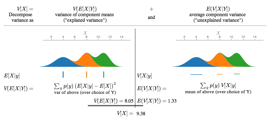
The law of total variance is a fundamental result in probability theory that expresses the variance of a random variable Y in terms of its conditional variances and conditional means given another random variable X. Informally, it states that the overall variability of Y can be split into an “unexplained” component (the average of within-group variances) and an “explained” component (the variance of group means).

Formally, if X and Y are random variables on the same probability space, and Y has finite variance, then:

$${\displaystyle \operatorname {Var} (Y)\;=\;\operatorname {E} {\bigl [}\operatorname {Var} (Y\mid X){\bigr ]}\; \;\operatorname {Var} \!{\bigl (}\operatorname {E} [Y\mid X]{\bigr )}.\!}$$

This identity is also known as the variance decomposition formula, the conditional variance formula, the law of iterated variances, or colloquially as Eve’s law, in parallel to the “Adam’s law” naming for the law of total expectation.

In actuarial science (particularly in credibility theory), the two terms ${\displaystyle \operatorname {E} [\operatorname {Var} (Y\mid X)]}$ and ${\displaystyle \operatorname {Var} (\operatorname {E} [Y\mid X])}$ are called the expected value of the process variance (EVPV) and the variance of the hypothetical means (VHM) respectively.

Explanation

Let Y be a random variable and X another random variable on the same probability space. The law of total variance can be understood by noting:

1. ${\displaystyle \operatorname {Var} (Y\mid X)}$ measures how much Y varies around its conditional mean ${\displaystyle \operatorname {E} [Y\mid X].}$
2. Taking the expectation of this conditional variance across all values of X gives ${\displaystyle \operatorname {E} [\operatorname {Var} (Y\mid X)]}$, often termed the “unexplained” or within-group part.
3. The variance of the conditional mean, ${\displaystyle \operatorname {Var} (\operatorname {E} [Y\mid X])}$, measures how much these conditional means differ (i.e. the “explained” or between-group part).

Adding these components yields the total variance ${\displaystyle \operatorname {Var} (Y)}$, mirroring how analysis of variance partitions variation.

Examples

Example 1 (Exam Scores)

Suppose five students take an exam scored 0–100. Let Y = student’s score and X indicate whether the student is *international* or *domestic*:

• Mean and variance for international: ${\displaystyle \operatorname {E} [Y\mid X={\text{Intl}}]=50,\;\operatorname {Var} (Y\mid X={\text{Intl}})\approx 1266.7.}$
• Mean and variance for domestic: ${\displaystyle \operatorname {E} [Y\mid X={\text{Dom}}]=50,\;\operatorname {Var} (Y\mid X={\text{Dom}})=100.}$

Both groups share the same mean (50), so the explained variance ${\displaystyle \operatorname {Var} (\operatorname {E} [Y\mid X])}$ is 0, and the total variance equals the average of the within-group variances (weighted by group size), i.e. 800.

Example 2 (Mixture of Two Gaussians)

Let X be a coin flip taking values Heads with probability h and Tails with probability 1−h. Given Heads, Y ~ Normal(${\displaystyle \mu _{h},\sigma _{h}^{2}}$); given Tails, Y ~ Normal(${\displaystyle \mu _{t},\sigma _{t}^{2}}$). Then ${\displaystyle \operatorname {E} [\operatorname {Var} (Y\mid X)]=h\,\sigma _{h}^{2} (1-h)\,\sigma _{t}^{2},}$ ${\displaystyle \operatorname {Var} (\operatorname {E} [Y\mid X])=h\,(1-h)\,(\mu _{h}-\mu _{t})^{2},}$ so ${\displaystyle \operatorname {Var} (Y)=h\,\sigma _{h}^{2} (1-h)\,\sigma _{t}^{2}\; \;h\,(1-h)\,(\mu _{h}-\mu _{t})^{2}.}$

Example 3 (Dice and Coins)

Consider a two-stage experiment:

1. Roll a fair die (values 1–6) to choose one of six biased coins.
2. Flip that chosen coin; let Y=1 if Heads, 0 if Tails.

Then ${\displaystyle \operatorname {E} [Y\mid X=i]=p_{i},\;\operatorname {Var} (Y\mid X=i)=p_{i}(1-p_{i}).}$ The overall variance of Y becomes ${\displaystyle \operatorname {Var} (Y)=\operatorname {E} {\bigl [}p_{X}(1-p_{X}){\bigr ]} \operatorname {Var} {\bigl (}p_{X}{\bigr )},}$ with ${\displaystyle p_{X}}$ uniform on ${\displaystyle \{p_{1},\dots ,p_{6}\}.}$

Proof

Discrete/Finite Proof

Let ${\displaystyle (X_{i},Y_{i})}$, ${\displaystyle i=1,\ldots ,n}$, be observed pairs. Define ${\displaystyle {\overline {Y}}=\operatorname {E} [Y].}$ Then ${\displaystyle \operatorname {Var} (Y)={\frac {1}{n}}\sum _{i=1}^{n}{\bigl (}Y_{i}-{\overline {Y}}{\bigr )}^{2}={\frac {1}{n}}\sum _{i=1}^{n}{\Bigl [}(Y_{i}-{\overline {Y}}_{X_{i}}) ({\overline {Y}}_{X_{i}}-{\overline {Y}}){\Bigr ]}^{2},}$ where ${\displaystyle {\overline {Y}}_{X_{i}}=\operatorname {E} [Y\mid X=X_{i}].}$ Expanding the square and noting the cross term cancels in summation yields: ${\displaystyle \operatorname {Var} (Y)=\operatorname {E} {\bigl [}\operatorname {Var} (Y\mid X){\bigr ]}\; \;\operatorname {Var} \!{\bigl (}\operatorname {E} [Y\mid X]{\bigr )}.\!}$

General Case

Using ${\displaystyle \operatorname {Var} (Y)=\operatorname {E} [Y^{2}]-\operatorname {E} [Y]^{2}}$ and the law of total expectation: ${\displaystyle \operatorname {E} [Y^{2}]=\operatorname {E} {\bigl [}\operatorname {E} (Y^{2}\mid X){\bigr ]}=\operatorname {E} {\bigl [}\operatorname {Var} (Y\mid X) \operatorname {E} [Y\mid X]^{2}{\bigr ]}.}$ Subtract ${\displaystyle \operatorname {E} [Y]^{2}={\bigl (}\operatorname {E} [\operatorname {E} (Y\mid X)]{\bigr )}^{2}}$ and regroup to arrive at ${\displaystyle \operatorname {Var} (Y)=\operatorname {E} {\bigl [}\operatorname {Var} (Y\mid X){\bigr ]} \operatorname {Var} \!{\bigl (}\operatorname {E} [Y\mid X]{\bigr )}.\!}$

Applications

Analysis of Variance (ANOVA)

In a one-way analysis of variance, the total sum of squares (proportional to ${\displaystyle \operatorname {Var} (Y)}$) is split into a “between-group” sum of squares (${\displaystyle \operatorname {Var} (\operatorname {E} [Y\mid X])}$) plus a “within-group” sum of squares (${\displaystyle \operatorname {E} [\operatorname {Var} (Y\mid X)]}$). The F-test examines whether the explained component is sufficiently large to indicate X has a significant effect on Y.

Regression and R²

In linear regression and related models, if ${\displaystyle {\hat {Y}}=\operatorname {E} [Y\mid X],}$ the fraction of variance explained is ${\displaystyle R^{2}={\frac {\operatorname {Var} ({\hat {Y}})}{\operatorname {Var} (Y)}}={\frac {\operatorname {Var} (\operatorname {E} [Y\mid X])}{\operatorname {Var} (Y)}}=1-{\frac {\operatorname {E} [\operatorname {Var} (Y\mid X)]}{\operatorname {Var} (Y)}}.}$ In the simple linear case (one predictor), ${\displaystyle R^{2}}$ also equals the square of the Pearson correlation coefficient between X and Y.

Machine Learning and Bayesian Inference

In many Bayesian and ensemble methods, one decomposes prediction uncertainty via the law of total variance. For a Bayesian neural network with random parameters ${\displaystyle \theta }$: ${\displaystyle \operatorname {Var} (Y)=\operatorname {E} {\bigl [}\operatorname {Var} (Y\mid \theta ){\bigr ]} \operatorname {Var} {\bigl (}\operatorname {E} [Y\mid \theta ]{\bigr )},}$ often referred to as “aleatoric” (within-model) vs. “epistemic” (between-model) uncertainty.

Actuarial Science

Credibility theory uses the same partitioning: the expected value of process variance (EVPV), ${\displaystyle \operatorname {E} [\operatorname {Var} (Y\mid X)],}$ and the variance of hypothetical means (VHM), ${\displaystyle \operatorname {Var} (\operatorname {E} [Y\mid X]).}$ The ratio of explained to total variance determines how much “credibility” to give to individual risk classifications.

Information Theory

For jointly Gaussian ${\displaystyle (X,Y)}$, the fraction ${\displaystyle \operatorname {Var} (\operatorname {E} [Y\mid X])/\operatorname {Var} (Y)}$ relates directly to the mutual information ${\displaystyle I(Y;X).}$ In non-Gaussian settings, a high explained-variance ratio still indicates significant information about Y contained in X.

Generalizations

The law of total variance generalizes to multiple or nested conditionings. For example, with two conditioning variables ${\displaystyle X_{1}}$ and ${\displaystyle X_{2}}$: ${\displaystyle \operatorname {Var} (Y)=\operatorname {E} {\bigl [}\operatorname {Var} (Y\mid X_{1},X_{2}){\bigr ]} \operatorname {E} {\bigl [}\operatorname {Var} (\operatorname {E} [Y\mid X_{1},X_{2}]\mid X_{1}){\bigr ]} \operatorname {Var} (\operatorname {E} [Y\mid X_{1}]).}$ More generally, the law of total cumulance extends this approach to higher moments.

See also

• Law of total expectation (Adam’s law)
• Law of total covariance
• Law of total cumulance
• Analysis of variance
• Conditional expectation
• R-squared
• Fraction of variance unexplained
• Variance decomposition

References

• Blitzstein, Joe. "Stat 110 Final Review (Eve's Law)" (PDF). stat110.net. Harvard University, Department of Statistics. Retrieved 9 July 2014.
• "Law of total variance". The Book of Statistical Proofs.
• Billingsley, Patrick (1995). "Problem 34.10(b)". Probability and Measure. New York, NY: John Wiley & Sons, Inc. ISBN 0-471-00710-2.
• Weiss, Neil A. (2005). A Course in Probability. Addison–Wesley. pp. 380–386. ISBN 0-201-77471-2.
• Bowsher, C.G.; Swain, P.S. (2012). "Identifying sources of variation and the flow of information in biochemical networks". PNAS. 109 (20): E1320 – E1328. doi:10.1073/pnas.1118365109.